Objectives: By the end of this subtopic learners should be able to:
Classify and interpret symbols on a map.
Describe the importance of a key.
Identify and use the different types of scale.
Use coordinates to locate places on a map.
Measure distances accurately on a map.
Calculate direction and bearing on a map.
Draw and interpret sketch maps.
Recognize various features represented by contour lines on maps.
A Map
Definition Of Map:
A map is a representation of physical and human features of an area of the earth's surface drawn to scale on a flat plane or piece of paper.
Features represented on a map are both natural (relief, water, vegetation) and man-made (buildings, roads and other landuse)
Topocadastral Maps
A topographical map is a map that shows relief, water and vegetation features of an area.
Topocadastral maps are maps that show both topographical features of an area as well as additional information such as farm boundaries.
The main type of map used in Zimbabwe's school system is the 1:50000 topocadastral or topographic map.
Atlas
This is a book of maps.
It contains many types of maps presented in different scales.
Map symbols and references
Symbols
Maps, unlike photographs, use symbols to represent actual features.
These symbols are generally agreed by cartographers (map makers).
Map symbols are classified into two groups: those representing physical features and those representing human features.
Symbols of physical features
Symbols of physical features are further subdivided into water, relief and vegetation.
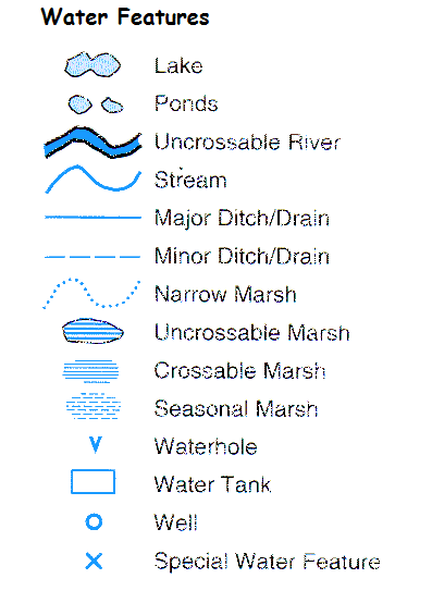
Water features
All water features are represented on a map with the associative colour blue.
The water features may be natural such as streams, springs and marsh or manmade such as dams, water tanks and canals.
In the presentation of symbols below water features are shown in their colour blue.
Water Features
Although not all of the water features may be memorised, it is important to keep familiarity with the following: small stream, river, waterfall, rapid, well, borehole, dam, reservoir and marsh.
TASK:
Identify from the key given below and reproduce, by drawing, the above named water features in your exercise books.
KEY
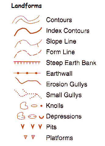
These are represented in brown.
The simplest brown line is a contour.
The various contour patterns tell us which feature there is on the map and this requires some set of map reading skills.
Contour patterns are discussed further later on in this section of map skills.
In the key given below there are a number of relief features that can be found on a topographical map.
Relief Features
These are represented in brown
The simplest brown line is a contour.
The various contour patterns tell us which feature there is on the map and this requires some set of map reading skills.
In the key given above there are a number of relief features that need to be read carefully.
These can be further compared to another set of symbols given below.
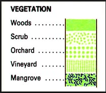
Vegetation Features
Vegetation features are represented in green colour.
The green colour can be of different hue to denote differences in density.
In Zimbabwe, we usually use four broad classifications namely: dense bush, medium bush, sparse bush or open grassland and plantation or orchard.
In the key below are some vegetation features symbols.
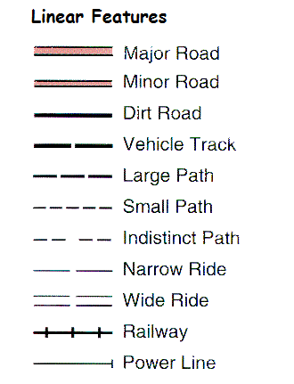
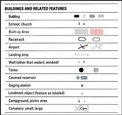
Human Features
These are physical features built by humans and they constitute the broadest class.
They are mostly represented in black although a variety of other colours may be used to give prominence to some phenomenon.
Red is usually used to represent roads and boundaries.
The main key given earlier shows the different classes of human features symbols.
One can compare those to the small extract given below.
near Features
Buildings and related features
The Key
The internationally agreed map symbols only provide a guide but more representation of features goes into map making.
A key is thus important.
It is a guide to symbols used on a map.
A key is usually placed in a corner outside the map.
The key must contain symbols that clearly resemble those used inside the map in terms of basic shape/character and colour.
The word ‘key' must be clearly labeled on top.
Every map must have an accompanying key.
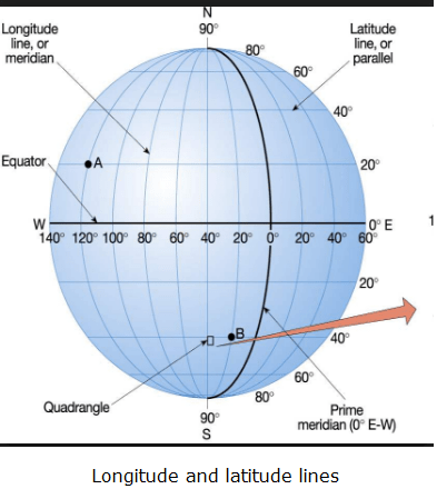
Location on maps
Longitude and latitude
Location on maps is done using different means that include use of grid reference, direction and bearing.
Longitudes are a set of imaginary lines drawn on the earth's surface for the purposes of locating places.
They run from the North Pole to the South Pole.
Longitudes are used together with latitudes which are lines drawn parallel to the Equator.
Longitude is the angular distance of a place on the earth's surface to the Greenwich meridian also known as prime meridian (see globe below).
Location of places is thus made with reference to either longitude or latitude as is indicated on the globe above.
In locating a place we quote the longitude immediately on the left or west and then latitude immediately below.
Further insight into location and time zones using longitudes and latitudes is tackled under transport studies.
Grid reference
Grid referencing
This is a system that uses vertical and horizontal lines on maps.
These lines are imaginary and do not have any relationship with features on the map and neither do they have anything to do with longitudes and latitudes.
Horizontal lines are called northings and they count from bottom to the top (for example 46 to 49 on the map extract below).
They count towards the north of the map and for that reason they are referred to as northings.
Vertical lines are called eastings and they count from the left of the page to the right or east (for example 28 to 31 below).
Grid referencing is done using four figure and six figure techniques.
Four figure grid reference
We indicate Easting (immediately to the left in the box where the feature is) first then Northing (immediately below).
Four figure grid of A is Easting 28 and Northing 48 giving 2848.
For B it is 2947 and C 3048.
Six figure grid reference
On the six figure grid system we quote Easting immediately to the left on a scale of one to ten towards the next easting to the right and northing immediately below and its distance towards the next northing above.
‘A' is thus on Easting 285 and northing 485.
Six figure grid reference of A is 285485.
‘B' is 291473 and ‘C' is 307487.
One very important skill in determining exact position is that of estimating correctly distances on a scale of one to ten.
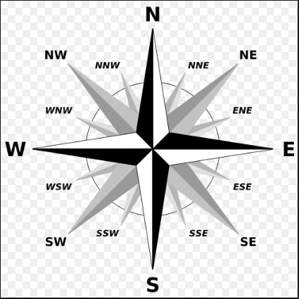
Direction
Compass points
Using cardinal and intercardinal points, general location of features can be made on a map.
Intercardinal or ordinal points are the eight or sixteen compass points as given below.
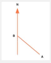
When telling the direction of one place from the other e.g. A from B, we start at B as shown in the diagram below.
A from B
We draw a north-south line at B and connect B to A with a line.
We are thus able to estimate the direction of A as south east.
Compass points are good in that they are easy and fast to use since they do not entail measurement.
They also use the skill of generalization.
On a map, the method is most useful in describing location of expansive areas.
Its weakness is in the fact that exactness or pin point accuracy of a location is difficult to arrive at.
It is not very useful in locating points.
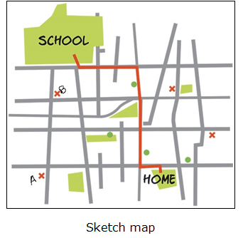
Using the sketch map below, direction is useful in locating the school and home which do not happen to be points.
The school is in the north-west (NW) while the home is in the south-east (SE) of the map.
Accuracy is, however, demanded in locating points A and B on the map in general as well as in relation to each other.
Sketch Map
Using bearing is the other way of enhancing use of compass points when locating places.
Bearing
Measurement of bearing is a skill that is extensively covered in mathematics.
It involves the use of both compass points and angles.
Bearing gives location of a place in relation to another place.
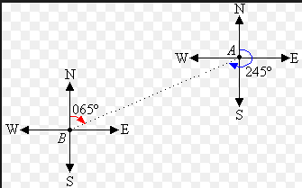
An example is the location of B from the position of A.
Telling the bearing of B from A involves drawing a north south line at A.
We draw a straight line from A to B.
The bearing of B from A is the angle of B on the north-south line from A.
Please note that in this case we use the Grid North.
We then measure the angle between the north-south line and the line joining A to B using a compass.
Bearing is thus 245°.
If we want the bearing of A from B, again we measure from B the angle of A on the north-south line which is 065°.
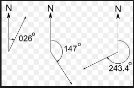
Below is an example of the different angles that can be measured to give bearing of a place.
Please note that in all cases the grid north is the one used.
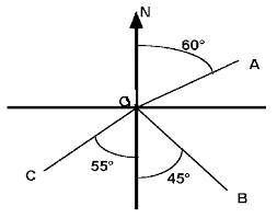
Bearing can be given as combination of both compass direction and angle.
In the diagram below A is from the north 60° towards the east (N60°E).
C is from the south 55° towards the west (S55°W).
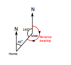
Reverse or back bearing
If we move from one point to another we are able to calculate bearing.
However, if we return to where we came from we are using reverse bearing.
It is reverse because we make a 180° turn to get back to where we were.
Reverse bearing is derived by adding 180° to our initial bearing if it is below 180° or subtracting 180° if it is above 180°.
reverse
In the above illustration bearing of school from home is 40°.
Reverse bearing is thus 40° + 180° = 220°.
If our initial bearing from a place is 260° then our reverse bearing will be 260° — 180° = 80°.
In the second case, our initial bearing is above 180° so we subtract 180°.
Using distance, direction and/or bearing we are able to follow description of routes on maps.
Scale
A map represents the earth's surface on a piece of paper.
This means that the distance on a map only represents the actual distance on the ground.
Scale is the ratio of distance on a map to the actual distance on the ground.
Scale is the extent to which the actual distance has been reduced so that it is represented on a map.
Types of scale
There are three types of scale: statement, representative fraction/ratio and linear scale.
Statement
This is in the form of a descriptive statement such as "one centimeter represents half a kilometer" or "1 centimeter represents 50 000 centimeters."
Representative fraction or ratio
It comes as a fraction or ratio such as 1/50000 or 1:50 000.
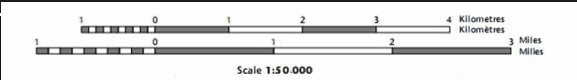
Linear
Scale is shown as a line with the first part divided into ten units (extension scale) and the second (primary scale) which if you measure with a ruler will show that 1 cm represents half a kilometer.
Small scale and large scale maps
The scale of a map is given by the size of the fraction.
When we say 1â„25 000 map is bigger than 1:50 000 map, it is because the fraction 1â„(25 000) has greater value than 1â„(50 000).
Most students confuse higher denominator with higher value.
The higher the denominator the smaller the fraction and therefore the smaller the map.
A small scale map is a map that has a fraction smaller than 1:50 000, for example 1:100 000.
Medium scale maps are between 1:50 000 and 1:25 000.
Large scale maps are those with scales larger than 1:25 000 such as 1:10 000.
Zimbabwean school system normally uses the 1:50 000 topographic map.
Measuring distance
We measure straight lines with a ruler.
We divide our measured distances (cm) with our representative fraction (e.g. 1:50000).
If we measure distance of 16cm on a map, actual distance on the ground will be:16 / (1â„50 000)= 32km.
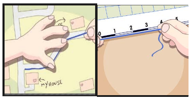
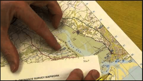
The challenge of measuring distances on a map comes when we measure curved distances.
One simple way is to use a string to follow through all bends and then straighten it up on a ruler to get straight line distance.
This is shown in the picture below:
Another method is that of using a piece of paper.
The paper is turned around as markings are done on all straight distances on both the paper and the map until the whole length that is measured is covered.
The markings on the piece of paper are then put against a ruler to measure straight line distance.
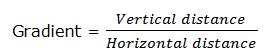
Gradient
It is generally described as the degree of slope.
It is the relationship between horizontal (run) and vertical (rise/fall) distance.
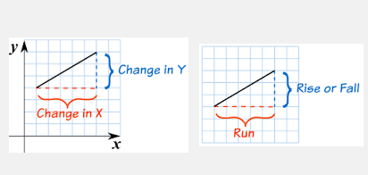
If we look at a simple diagram like one below gradient is given by yâ„x
If we regard boxes in the graph as centimeters then it will be3â„5= 0.6
What it means is that the ground rises by 0.6 cm per every horizontal distance of 1cm.
When this is applied to a map, horizontal distance is straight line distance between two points which can be measured with a ruler.
Vertical distance or height is calculated by finding difference in height between contours.
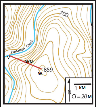
Using diagram above horizontal distance is from V to W = 3km.
Vertical distance is the difference between contours which is 859m-680m = 179m.
Next step is to convert both distances into similar units.
Height = 179m and horizontal distance =3000m.
Gradient is thus 179â„3000= 0.05966 = 59.67m/km.
For every kilometer there is a rise in the ground of 59.67 meters.
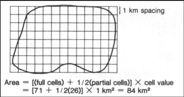
Estimating area on a map
Area is generally calculated by multiplying length by width.
However, this may be very taxing given irregular dimensions of most areal aspects of a map such as farmland, cultivated area, a game park, dam and so on.
A method of estimation is thus used.
Grid lines provide squares of 2cm by 2cm on a topocadastral map of 1:50 000.
Because 2cm represent 1 km, it means a box represents 1km².
Total area will thus be the sum of full boxes plus all estimate parts.
The illustration below gives us total area of 84km².
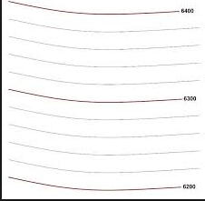
Contour lines
These are lines drawn on a map joining places of the same height above sea level.
Contour lines do not cross.
They may come close to each other or even merge where slopes are very steep like on cliffs.
The difference between two successive contour lines is called contour interval (CI).
On the topographical 1:50 000 map mostly used in schools in Zimbabwe the contour interval is 20m.
Labelling of contours is done on the contour lines themselves and in most cases every fifth contour that is bold has the label.
The labelled contour such as the 1000m one on the map below is known as an index contour.
Contour lines are brown in colour.
Advantages of using contour lines
Contour lines do not obscure any other detail on the map.
They are the most effective method of representing features, steepness or gentleness of the land.
Can be used together with spot heights, benchmarks and trigonometrical beacons where exact /specific heights are needed.
Can be used with layer colouring to classify or distinguish heights.
Spot height
These are dots on a map that mark specific height of a spot.
They only exist on maps and not physically on land.
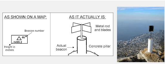
Trigonometrical beacon
These are stations marked on a map as well as on the ground.
They indicate the highest point in an area.
On the map they are presented in the form of a small triangle that has a specified height beside them.
They can, however, be numbered, for example 1200T.
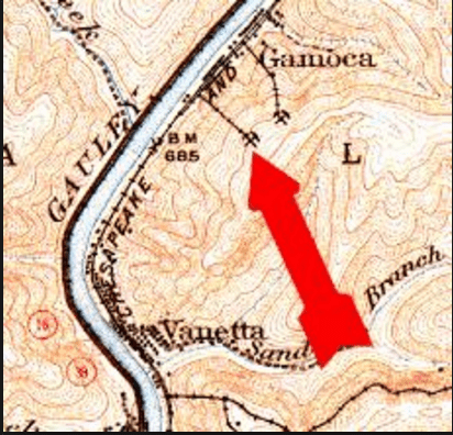
Benchmarks
A benchmark is normally a metal plug that is cast in concrete on the ground and has height engraved on it.
Contour lines, slopes and common landforms
Patterns of contours indicate the types of landscapes.
When contours are far apart land is gentle and when they are close together slopes are steep.
Gentle slope
The first contour diagram shows gentle slope while the second shows steep slope.
Steep slope
A map that has mostly even ground is seen by its sparse contours while hilly areas have predominantly close contours.
Even slope
Slopes are even when contours are evenly spaced and this is common with gentle slopes.
The illustration below shows an even contour pattern.
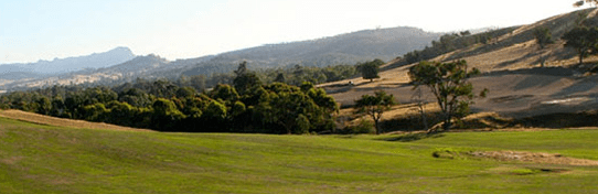
Undulating slope
A series of gentle up and down slopes give us an undulating landscape or slope.
The photograph and map below shows one such landscape.
Convex slopes
These are slopes that are gentle towards the top but steeper towards the bottom.
Contours start off far apart at the top becoming closer to each other towards the bottom as shown in the illustration below.
Concave slopes
Concave slopes are slopes that are steep at the top becoming gentle towards the bottom.
Contours are therefore close towards the summit but far apart at the bottom or base.
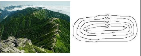
A Ridge
A ridge is an extended highland or mountain with a narrow top.
In Zimbabwe ridges are common along The Great Dyke and Eastern Highlands.
Below is a picture showing a ridge and its contour mapping.
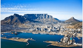
Plateau
It is also spelt as plateaux.
A plateau is a highland or mountain with a flat top.
A world example is found in South Africa named The Table Mountain.
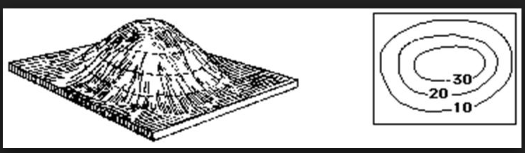
Conical hill
This is simply a round shaped hill.
The illustrations below show the side view as well as contour pattern.
Escarpment
An escarpment is a sudden fall of land caused by erosion or vertical movement of the earth's crust.
In Zimbabwe we have the Zambezi escarpment in north eastern parts of the country.
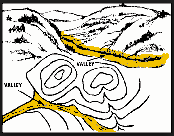
A Valley
A valley is an elongated lowland between highlands whose bottom is indicated by V or U shaped contours.
The formation of the V and U shaped valleys is extensively covered under rivers features.
Valley and spur
A spur is a highland jutting into a lowland or valley.
Spurs are often found interceded by narrow valleys as shown in the diagram below.
Gorge
This is a narrow river valley with deep but steep sides.
At Victoria Falls we have the famous Devils' gorge.
More discussion of it is done under landform studies.
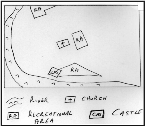
Sketch map
A sketch map is a map drawn from observation showing outline of features on the main map.
There are no actual measurements and concentration is given to
the aspects that need to be mapped ignoring other not so important ones.
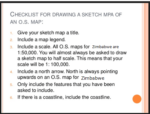
Drawing a sketch map
Obtain a base map.
Draw a frame of half the scale (1:100 000).
Draw the features that you want to focus on, for example, rivers, hilly areas, fields, grasslands and so on
Start with rivers, then hilly areas and lastly man-made features.
Shading is used to indicate areas while other features may be
represented by simple illustrations (for example roads and rivers).
Include a title and key or legend.
Indicate the grid north.
The steps are summarized below on a checklist of sketch map drawing.
Checklist fo sketch map drawing
Checlist of sketch map drawing
Drawing of sketch maps is a skill that is best mastered by constant practice.